Within-host \(\pi_W\)#
This code examines the frequency distribution of within-host nucleotide diversity \(\pi_W\) in samples taken from malaria-infected individuals around the world.
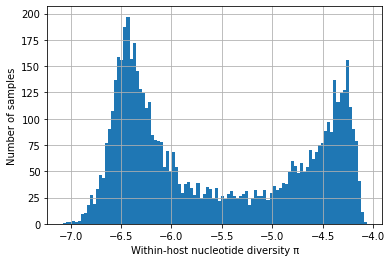
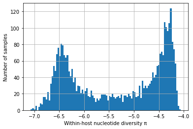
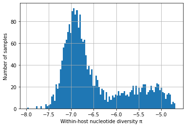
We find that \(\pi_W\) has a strikingly bimodal distribution (scroll down to see plots showing this).
We postulate that one of the peaks (with high \(\pi_W\)) represents hosts that have been superinfected, or who lie on a transmission chain where there is cotransmission following a recent episode of superinfection.
We postulate that the other peak (with low \(\pi_W\)) represents transmission chains where there has been no recent superinfection or cotransmission.
We can use the low \(\pi_W\) peak to estimate the quantum of transmission with the formula \(Q = \pi_W / 2 \mu\).
About the data#
Data are from the MalariaGEN Pf6 dataset which has data on 6,051,696 variants in 7,113 samples from 30 countries. This notebook uses files that we have created based on:
Selected variants that are high-quality biallelic coding SNPs (n = 502,221). High quality means ‘filter_pass == True’ & ‘vqslod > 3’
Selected samples that passed QC (n = 5,970)
Data on allele depth for reference and non-reference forms of these biallelic SNPs in individual samples, from which we have calculated within-host heterozygosity for each SNP in each sample.
Elsewhere we show an analysis of the SNPs that are heterozygous in samples with low \(\pi_W\) as a sanity check to exclude the possibility that the low \(\pi_W\) peak is a technical artefact due to systematic genotyping errors.
We will use these files#
These files are not currently available via Google Colab so this notebook is for info only
wiho_het.npy
Gives within-host heterozygosity for each SNP (n = 502,221) in each sample (n = 5,970).
As we have selected biallelic SNPs this is easy to calculate from allele depth data.
Filename:
230318_wiho_het.npyThis is a large file - 11.7GB - so it takes a while to process
region
A list of geographical regions for 5,970 selected samples
‘SAM’=South America, ‘WAF’=West Africa, ‘CAF’=Central Africa, ‘EAF’=East African, ‘SAS’=South Asia, ‘WSEA’=Western SE Asia, ‘ESEA’=Eastern SE Asia, ‘OCE’=Oceania
Filename:
230316_region
het_per_snp
Mean within-host heterozygosity for each SNP, calculated from
wiho_het.npyFilename:
230317_het_per_snp
het_per_sample
Mean within-host heterozygosity for each sample after filtering by SNP heterozygosity (typically <0.02) and by geographical region.
Filenames:
All regions (5970 samples):
230317_het_per_sample_ALLSoutheast Asia:
230316_het_per_sample_SEAAfrica (3314 samples):
230317_het_per_sample_Africa
# This code currently requires the above files to be mounted on the user's Google Drive

from google.colab import drive

drive.mount('/content/drive')

data_path = "/content/drive/My Drive/Colab Data/Pf6/"
Mounted at /content/drive
import numpy as np
import json
import math
import matplotlib.pyplot as plt
import statistics as stat
selected_snps = 502221
selected_samples = 5970
Create snp_filter to filter out possible hyperhets#
Here we use het < 0.02 as our criterion for inclusion
with open(data_path + "230317_het_per_snp", "r") as fp:
    het_per_snp = json.load(fp)

snp_filter = []

for i in range(selected_snps):

    if het_per_snp[i] < 0.02:

        snp_filter.append(True)

    else:
        snp_filter.append(False)

filtered_snps = snp_filter.count(True)

print('This includes', str(filtered_snps), 'SNPs')
This includes 496459 SNPs
Create sample_filter to select a particular geographical region#
‘SAM’=South America, ‘WAF’=West Africa, ‘CAF’=Central Africa, ‘EAF’=East African, ‘SAS’=South Asia, ‘WSEA’=Western SE Asia, ‘ESEA’=Eastern SE Asia, ‘OCE’=Oceania
with open(data_path + "230316_region", "r") as fp:
    region = json.load(fp)

sample_filter = []

for i in range(selected_samples):

    if region[i] == "CAF" or region[i] == "EAF" or region[i] == "WAF":

        sample_filter.append(True)

    else:

        sample_filter.append(False)

filtered_samples = sample_filter.count(True)

print('This includes', str(filtered_samples), 'samples')
This includes 3314 samples
Calculate mean heterozygosity per sample after filtering samples and SNPs#
Creates a list of het values, one for each selected & filtered sample
This is the mean het for selected & filtered SNPs and not for all nucleotide positions
On Colab this should take approximately 15 minutes depending on the selection of regions
Save the output for future use
wiho_het = np.load(data_path + '230318_wiho_het.npy', mmap_mode = 'r')

het_per_sample = []

for i in range(selected_samples):

    if sample_filter[i] == True:

        het = []

        for j in range(selected_snps):

            if snp_filter[j] == True:

                het.append(wiho_het[j, i])

        y = stat.mean(het)

        het_per_sample.append(y)

    if i % 10 == 0:

        print(i)

with open(data_path + "230317_het_per_sample_Africa", "w") as filepath:
    json.dump(het_per_sample, filepath)
Plot histogram of within-host nucleotide diversity#
# All regions - only SNPs with het < 0.02

with open(data_path + "230317_het_per_sample_ALL", "r") as filepath:
    het_per_sample = json.load(filepath)

selected_snps = 496459 # this is <0.02 het, total SNPs is 502221
coding_positions = 12028350 # from Gardner et al 2002

convert_het_to_pi = selected_snps / coding_positions

het_per_sample_nonzero = [convert_het_to_pi * x for x in het_per_sample if x != 0]
log_het_per_sample = [math.log(x, 10) for x in het_per_sample_nonzero]
plt.hist(log_het_per_sample, bins = 100)
plt.xlabel('Within-host nucleotide diversity \u03C0')
plt.ylabel('Number of samples')
plt.grid()
plt.show()

# Africa - only SNPs with het < 0.02

with open(data_path + "230317_het_per_sample_Africa", "r") as filepath:
    het_per_sample = json.load(filepath)

selected_snps = 496459 # this is <0.02 het, total SNPs is 502221
coding_positions = 12028350 # from Gardner et al 2002

convert_het_to_pi = selected_snps / coding_positions

het_per_sample_nonzero = [convert_het_to_pi * x for x in het_per_sample if x != 0]
log_het_per_sample = [math.log(x, 10) for x in het_per_sample_nonzero]
plt.hist(log_het_per_sample, bins = 100)
plt.xlabel('Within-host nucleotide diversity \u03C0')
plt.ylabel('Number of samples')
plt.grid()
plt.show()

# Southeast Asia - only SNPs with het < 0.02

with open(data_path + "230316_het_per_sample_SEA", "r") as filepath:
    het_per_sample = json.load(filepath)

selected_snps = 496459 # this is <0.02 het, total SNPs is 502221
coding_positions = 12028350 # from Gardner et al 2002

convert_het_to_pi = selected_snps / coding_positions

het_per_sample_nonzero = [convert_het_to_pi * x for x in het_per_sample if x != 0]
log_het_per_sample = [math.log(x, 10) for x in het_per_sample_nonzero]
plt.hist(log_het_per_sample, bins = 100)
plt.xlabel('Within-host nucleotide diversity \u03C0')
plt.ylabel('Number of samples')
plt.grid()
plt.show()


