get_coalescent#
Once we have created a population by specifying its transmission history, it is very simple to perform a Markov chain simulation of coalescence times by invoking get_coalescent.
!pip install coalestr
from coalestr import cs
# Specify the transmission history of a population
# Each inner list gives [duration, N, Q, X, M] for a period of history
my_history = [[1000, 30, 10, 0, 0], [1000, 10, 5, 0.5, 0]]

# Create the population
my_population = cs.Population(my_history)

# Obtain coalescence times
my_population.get_coalescent()
Observation time.    Events captured.   Mean coalescence time
                      beho      wiho        beho     wiho
        0             100.0     100.0        25.1     18.9
Mean coalescence time
The ‘beho’ or between-host column on the right tells us that two alleles sampled from different hosts have a mean coalescence time of 25.1 generations.
The ‘wiho’ or within-host column on the right tells us that two alleles sampled from the same host have a mean coalescence time of 18.9 generations.
Events captured
The ‘events captured’ columns tell us that 100% of coalescent events are captured for both the between-host and the within-host simulation. This is an important QC check because we want to be sure that our simulation runs for long enough to capture the vast majority of coalescent events.
Let us see what happens if we drastically reduce the duration of our population history.
my_history = [[30, 30, 10, 0, 0], [10, 10, 5, 0.5, 0]]

my_population = cs.Population(my_history)

my_population.get_coalescent()
Observation time.    Events captured.   Mean coalescence time
                      beho      wiho        beho     wiho
        0              68.6      77.2        10.7      8.4
Here we appear to have shorter coalescence times but the results are unreliable because we are capturing only 68.6% of coalescent events for the between-host simulation and 77.2% of coalescent events for the within-host simulation.
Observation times#
In the above examples we made a single observation of the population at observation time = 0. This means that we sampled two alleles at time = 0 and followed their lineages back in time until they coalesced. Since we are proceeding back in time, observation time 0 means the present, or the most recent generation in the population history.
If we want to see how the genetic diversity of the population changes over time, then we need to make observations at multiple time points. For example, we might make observations every 500 generations. We can do this by providing get_coalescent with a list of observation times, always remembering that we are counting in backwards time, so observation time = 500 means 500 generations before the present.
my_history = [[1000, 30, 10, 0, 0], [1000, 10, 5, 0.5, 0]]

my_observations = [0, 500, 1000, 1500]

my_population = cs.Population(my_history)

my_population.get_coalescent(observe = my_observations)
Observation time.    Events captured.   Mean coalescence time
                      beho      wiho        beho     wiho
        0             100.0     100.0        25.1     18.9
      500             100.0     100.0        25.1     18.9
     1000             100.0     100.0        39.0     10.0
     1500             100.0     100.0        39.0     10.0
# We can also give a range of observation times like this

my_observations = range(0, 2000, 500)

my_population.get_coalescent(observe = my_observations)
Observation time.    Events captured.   Mean coalescence time
                      beho      wiho        beho     wiho
        0             100.0     100.0        25.1     18.9
      500             100.0     100.0        25.1     18.9
     1000             100.0     100.0        39.0     10.0
     1500             100.0     100.0        39.0     10.0
# We can retrieve a list of observation times as a population attribute

my_population.observation_times
[0, 500, 1000, 1500]
Data objects#
get_coalescent generates various data objects that are used by get_diversity and other methods. For most purposes we can ignore these data objects, and simply focus on the reports that are automatically produced when we run get_coalescent or get_diversity. However if we want to take a deep dive into the results of the Markov chain simulation, we can retrieve these data objects as attributes of our population:
t_simreportbeho_lineagewiho_lineagecoalescent
t_sim gives the duration of the simulation. For a simple population without migration, t_sim = t_his which is the duration of the population history. For a subpopulation that is embedded in a metapopulation, where the population history of the metapopulation may be greater than that of the subpopulation, t_sim gives the duration of the metapopulation history.
report gives a summary of coalescence events for different observation times.
axis 0:
observation_times[i]axis 1: summary of coalescence events
0: observation time
1: beho: percentage of coalescent events captured
2: wiho: percentage of coalescent events captured
3: beho: expectation of coalescence time
4: wiho: expectation of coalescence_time
5: eco setpoint: proportion of coalescences to capture
6: break time
Here is an example of how we can use report.
for i in range(len(my_population.observation_times)):

    print("At observation time {0:1.0f} the mean time to coalescence was\
    \n   {1:1.1f} for a between-host sample ({2:1.0f}% events captured)\
    \n   {3:1.1f} for a within-host sample ({4:1.0f}% events captured)"
        .format(
        my_population.report[i, 0],
        my_population.report[i, 3],
        my_population.report[i, 1],
        my_population.report[i, 4],
        my_population.report[i, 2]))
At observation time 0 the mean time to coalescence was
   25.1 for a between-host sample (100% events captured)
   18.9 for a within-host sample (100% events captured)
At observation time 500 the mean time to coalescence was
   25.1 for a between-host sample (100% events captured)
   18.9 for a within-host sample (100% events captured)
At observation time 1000 the mean time to coalescence was
   39.0 for a between-host sample (100% events captured)
   10.0 for a within-host sample (100% events captured)
At observation time 1500 the mean time to coalescence was
   39.0 for a between-host sample (100% events captured)
   10.0 for a within-host sample (100% events captured)
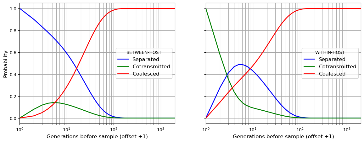
beho_lineage describes variation over time in the state of two lineages sampled from different hosts at observation time 0. This will allow us to estimate between-host levels of genetic diversity.
wiho_lineage describes variation over time in the state of two lineages sampled from the same host at observation time 0. This will allow us to estimate within-host levels of genetic diversity.
beho_lineage and wiho_lineage are both arrays with the following structure:
axis 0: backwards time
axis 1:
0: probability that lineages are separated
1: probability that lineages are cotransmitted
2: probability that lineages are coalesced
3: blank
4: blank
5: probability of coalescence occuring at this timepoint
6: summation series for expectation of coalescence time
Let us see how beho_lineage and wiho_lineage can be used to plot the state of two lineages going back in time for my_population created above.
import matplotlib.pyplot as plt

b_separated = my_population.beho_lineage[:, 0]
b_cotransmitted = my_population.beho_lineage[:, 1]
b_coalesced = my_population.beho_lineage[:, 2]

w_separated = my_population.wiho_lineage[:, 0]
w_cotransmitted = my_population.wiho_lineage[:, 1]
w_coalesced = my_population.wiho_lineage[:, 2]

timescale = range(1, my_population.t_his + 1)

fig, (ax1, ax2) = plt.subplots(1, 2, figsize=(14,5), sharex = True, sharey = True)

ax1.plot(timescale, b_separated, marker='', color='blue', linewidth = 2, label="Separated")
ax1.plot(timescale, b_cotransmitted, marker='', color='green', linewidth = 2, label="Cotransmitted")
ax1.plot(timescale, b_coalesced, marker='', color='red', linewidth = 2, label="Coalesced")

ax2.plot(timescale, w_separated, marker='', color='blue', linewidth = 2, label="Separated")
ax2.plot(timescale, w_cotransmitted, marker='', color='green', linewidth = 2, label="Cotransmitted")
ax2.plot(timescale, w_coalesced, marker='', color='red', linewidth = 2, label="Coalesced")

ax1.legend(title="BETWEEN-HOST",frameon=True, fontsize=12)
ax2.legend(title="WITHIN-HOST",frameon=True, fontsize=12)
ax1.set_xlabel("Generations before sample (offset +1)", fontsize=12)
ax2.set_xlabel("Generations before sample (offset +1)", fontsize=12)
ax1.set_ylabel("Probability", fontsize=12)
ax1.set_xscale('log',base=10)
ax1.set_xlim(1,my_population.t_his)
ax1.grid(visible=True, which='both', color='0.65', linestyle='-')
ax2.grid(visible=True, which='both', color='0.65', linestyle='-')

plt.show()

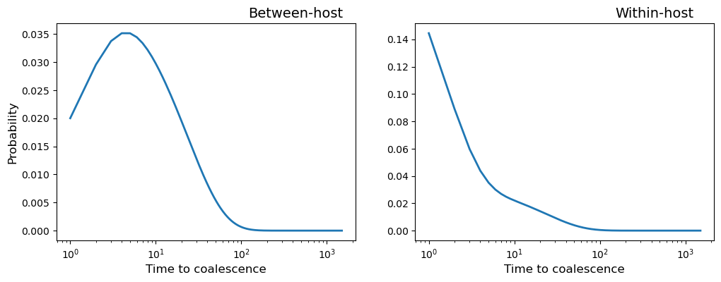
The population attribute coalescent describes the probability distribution of time to coalescence at different observation times. Recall that the population attribute observation_times is a list of observation times.
axis 0:
observation_times[i]axis 1: backwards time
axis 2: probability distribution of time to coalescence
0: beho: probability of coalescence occurring at this timepoint
1: wiho: probability of coalescence occurring at this timepoint
Let us see how this can be used to plot the probability distribution of coalescence times for observation time = 500.
obs_time = 500

i = my_population.observation_times.index(obs_time)

fig, (ax1, ax2) = plt.subplots(1, 2, figsize=(12,4), sharex = True)

timescale = range(1, my_population.t_his - obs_time)
beho_coalescent = my_population.coalescent[i, obs_time + 1:, 0]
wiho_coalescent = my_population.coalescent[i, obs_time + 1:, 1]

ax1.plot(timescale, beho_coalescent, marker='', linewidth=2)

ax2.plot(timescale, wiho_coalescent, marker='', linewidth=2)

ax1.set_title("Between-host", position=(0.8, 0.3), fontsize=14)
ax2.set_title("Within-host", position=(0.8, 0.3), fontsize=14)
ax1.set_xlabel("Time to coalescence", fontsize=12)
ax2.set_xlabel("Time to coalescence", fontsize=12)
ax1.set_ylabel("Probability", fontsize=12)
ax1.set_xscale('log',base=10)

plt.show()


