Hw - Hs relationship

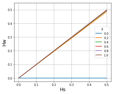
In regions of high malaria transmission there is considerable variation in within-host heterozygosity \(H_W\), depending on the frequency of superinfection and cotransmission. However when a very large number of SNP loci are analysed by deep genome sequencing of parasite samples from malaria-infected individuals, there is a striking linear correlation between \(H_W\) (the heterozygosity of a locus within an individual host) and \(H_S\) (the heterozygosity of that locus in the local subpopulation.

If \(\widehat{H}_W\) denotes the mean of \(H_W\) in the local subpopulation, we find that the slope of \(\widehat{H}_W/H_S\) (where \(H_S\) is the heterozygosity of the subpopulation) tends to increase with the malaria transmission intensity of the location. In the accompanying paper (link TBD) we derive the formula

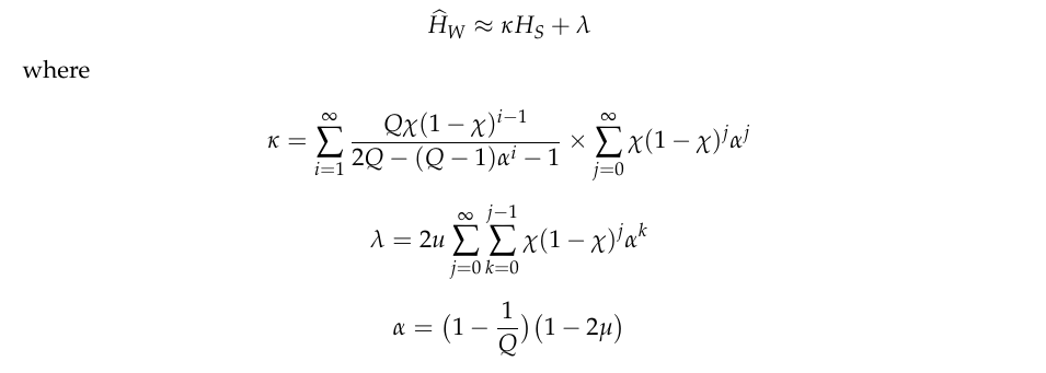
Here we use this formula to examine the relationship between \(\widehat{H}_W\) and \(H_S\) for different combinations of transmission parameters.

import matplotlib.pyplot as plt

# Plot Hw vs Hs for Q=1

Q = 1

X_list =  [x / 5 for x in range (6)]
Hs_list = [x / 20 for x in range(11)]
mu = 1.1e-8 # Mutation rate

alpha = (1 - 1 / Q) * (1 - 2 * mu) 

plt.figure(figsize = (6,5))

for X in X_list:
    
    Hw_list = []

    for Hs in Hs_list:
        
        sum1 = 0
        sum2 = X
        sum3 = 0
 
        for i in range(1, 100):

            sum1 += Q * X * (1 - X) ** (i - 1) / ( 2 * Q - (Q - 1) * alpha ** i - 1)
        
            sum2 += X * (1 - X) ** i * alpha ** i
        
        kappa = sum1 * sum2

        for j in range(0, 100):
        
            for k in range(0, j):
            
                sum3 += X * (1 - X) ** j * alpha ** k
            
        Lambda = 2 * mu * sum3
        
        Hw = kappa * Hs + Lambda    
        Hw_list.append(Hw)
    
    plt.plot(Hs_list, Hw_list, linewidth=2, label = X)
    
plt.xlabel("Hs", fontsize=16)
plt.ylabel("Hw", fontsize=16)
plt.ylim(top = 0.55)
plt.grid(visible=True, which='both', color='0.65', linestyle='-')
plt.legend(title="X", frameon=True) 

plt.show()

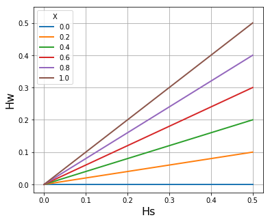
# Plot Hw vs Hs for Q=10

Q = 10

X_list =  [x / 5 for x in range (6)]
Hs_list = [x / 20 for x in range(11)]
mu = 1.1e-8 # Mutation rate
    
alpha = (1 - 1 / Q) * (1 - 2 * mu) 

plt.figure(figsize = (6,5))

for X in X_list:
    
    Hw_list = []

    for Hs in Hs_list:
        
        sum1 = 0
        sum2 = X
        sum3 = 0
 
        for i in range(1, 100):

            sum1 += Q * X * (1 - X) ** (i - 1) / ( 2 * Q - (Q - 1) * alpha ** i - 1)
        
            sum2 += X * (1 - X) ** i * alpha ** i
        
        kappa = sum1 * sum2

        for j in range(0, 100):
        
            for k in range(0, j):
            
                sum3 += X * (1 - X) ** j * alpha ** k
            
        Lambda = 2 * mu * sum3
        
        Hw = kappa * Hs + Lambda    
        Hw_list.append(Hw)
    
    plt.plot(Hs_list, Hw_list, linewidth=2, label = X)
    
plt.xlabel("Hs", fontsize=16)
plt.ylabel("Hw", fontsize=16)
plt.ylim(top = 0.55)
plt.grid(visible=True, which='both', color='0.65', linestyle='-')
plt.legend(title="X", frameon=True) 

plt.show()

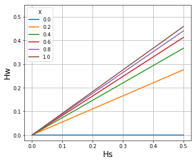
# Plot Hw vs Hs for Q=300

Q = 300

X_list =  [x / 5 for x in range (6)]
Hs_list = [x / 20 for x in range(11)]
mu = 1.1e-8 # Mutation rate

alpha = (1 - 1 / Q) * (1 - 2 * mu) 

plt.figure(figsize = (6,5))

for X in X_list:
    
    Hw_list = []

    for Hs in Hs_list:
        
        sum1 = 0
        sum2 = X
        sum3 = 0
 
        for i in range(1, 100):

            sum1 += Q * X * (1 - X) ** (i - 1) / ( 2 * Q - (Q - 1) * alpha ** i - 1)
        
            sum2 += X * (1 - X) ** i * alpha ** i
        
        kappa = sum1 * sum2

        for j in range(0, 100):
        
            for k in range(0, j):
            
                sum3 += X * (1 - X) ** j * alpha ** k
            
        Lambda = 2 * mu * sum3
        
        Hw = kappa * Hs + Lambda    
        Hw_list.append(Hw)
    
    plt.plot(Hs_list, Hw_list, linewidth=2, label = X)
    
plt.xlabel("Hs", fontsize=16)
plt.ylabel("Hw", fontsize=16)
plt.ylim(top = 0.55)
plt.grid(visible=True, which='both', color='0.65', linestyle='-')
plt.legend(title="X", frameon=True,loc=7) 

plt.show()